Using Bayesian Statistics to Identify Michigan COVID-19 Hot Spots

Datasets

New York Times COVID-19 Datasets

The New York Times provides a dataset containing a timeseries of the number of cases and deaths per county. The Federal Information Processing Standards (FIPS) code is a unique 5-digit identifier for each county. The FIPS code can be used to join with other datasets such as Census demographic data (e.g. population estimates).

The New York Times dataset provides the cumulative count of cases so I take the difference in cases to recover the daily count of cases per county. Then I take the sum of cases in the past two weeks as an estimate of the number of recent cases.

U.S. Census County Population

The tidycensus package provides access to U.S. Census Bureau data. In addition to Census demographic data the package provides county spatial geometries, which is useful for mapping. I use the tidycensus package to retrieve the 2018 American Community Survey (ACS) population estimate for each county and calculate the county-level COVID-19 incidence rate.

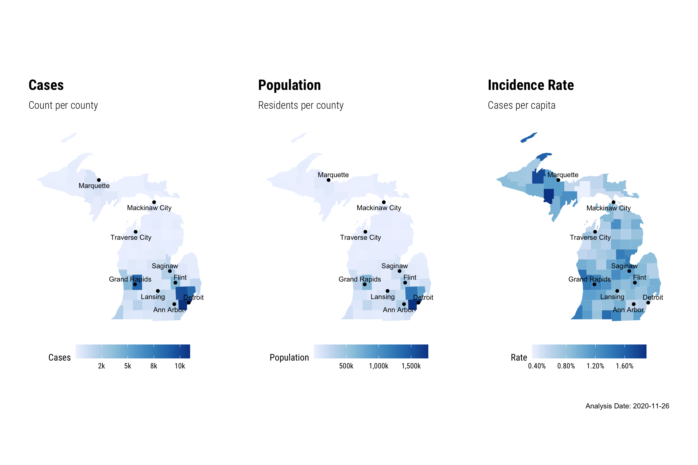
The maps below show the count recent COVID-19 cases per county (left), the county populations (center), and incidence rate (right). Notable cities are marked for reference. As you might expect the map of COVID-19 cases looks similar to the population map. This makes sense because we’d expect to see more COVID-19 cases where there are more people. Thus the incidence rate is a better measurement of risk.

Model

In order to estimate the county-level risk of COVID-19 I use a hierarchical beta-binomial model. The count of COVID-19 cases per county is taken to be a random draw from a binomial distribution with the number of trials being the county population with a certain probability. Given that we know the true count of COVID-19 cases per county and the county population, the aim of the model is to estimate the COVID-19 probability.

The county-level probability of COVID-19 can be estimated independently – meaning that each county’s probability is estimated separately. This would essentially construct separate models for each county-level risk. This approach is called a no pooling model because the probability for one county doesn’t take into account any information from other counties. However estimating each county’s probability separately would yield estimates with large variances because there is less data. By contrast a complete pooling method would estimate each county-level risk using the state-level risk and understate the variance.

Estimating the county-level probabilities using a hierarchical model treats them as draws from a beta distribution. This is called partial pooling and yields county-level probability estimates that are informed by others. Considering that you know the risk of one county you’d expect the risk level of another county to be similar (but not exactly the same).

I fit the model using Stan, a probabilistic programming language that can perform full Bayesian statistical inference with MCMC sampling. I run 5 Markov chains for 40,000 iterations, discarding the first 20,000 iterations as warm-up (i.e. burn-in). In order to prevent divergent transitions and to allow the sampler more execution time (if necessary), I set the target acceptance rate to 0.9 and the maximum tree depth to 15.

The Stan model code is below.

data {
  int<lower=0> n; // Number of counties
  int<lower=0> cases[n]; // Count of cases per county
  int<lower=0> population[n]; // County populations
}
parameters {
  real<lower=0, upper=1> phi; // State-level risk
  real<lower=1> kappa; // State-level concentration
  vector<lower=0, upper=1>[n] theta; // County-level risk
}
transformed parameters {
  real alpha = phi * kappa;
  real beta = (1 - phi) * kappa;
}
model {
  kappa ~ pareto(1, 1.5);
  theta ~ beta(alpha, beta);
  cases ~ binomial(population, theta);
}

Results

I assessed whether the Markov chains had converged for each parameter using R-hat, a measurement of the ratio of between- and within-chain variance. The parameter R-hat values were all below 1.05, indicating the 5 Markov chains had converged to the same parameter estimates. Additionally the effective sample sizes were large enough to indicate the parameter posterior quantities are reliable. There were 0 divergent transitions and E-BFMI indicated no pathological behavior.

The Bayesian modeling approach produces 100,000 samples (5 chains * 40,000 / 2) instead of a single point estimate for each parameter. Taken together the samples form a distribution, known as a posterior distribution. The median is a reasonable estimate for the parameter and the 95% posterior interval yields the range of plausible values for the parameter Thus we can compare the county-level risk posterior medians to the observed incidence rates.

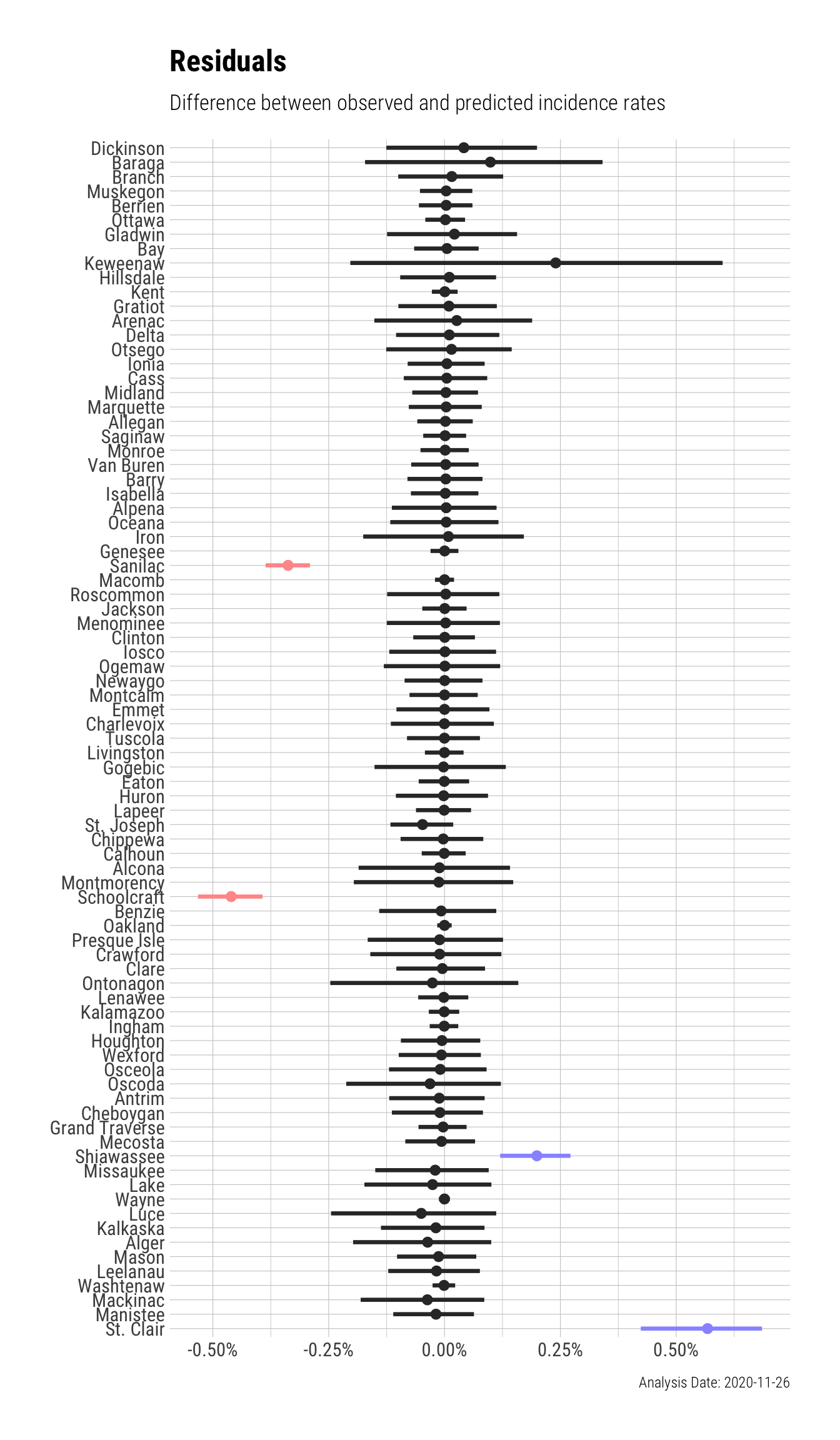
In statistics, differences between the observed and predicted value are called errors or residuals. Positive residuals represent that the model underestimated the risk – the observed value was greater than the predicted value. If the average of the residuals is significantly greater or lower than zero, then the model is systematically under or over estimating. In order to assess the model for this type of systematic error, we can check that the posterior interval contains the observed incidence rate. In this case there were 2 counties with overestimates, 2 counties with underestimates, and 79 counties without significant error.

The plot below shows the difference between the observed and predicted incidence rate 95% posterior intervals for each county. The posterior intervals that do not contain 0 (i.e. no difference) are underestimated (blue) or overestimated (red) by the model. Remember that positive residuals indicate underestimation and negative residuals indicate overestimation.

Public health officials are often interested in finding areas of elevated risks, often called clusters. The simplest method for identifying clusters is to impose a threshold and consider each area with a risk above the threshold as a cluster. The threshold can be based on an absolute value, such as a risk greater than 5%, or relative value, such as the top 10 counties with greatest risk.

In a Bayesian setting we can apply the threshold to any point of the posterior distribution. For example, we could find the probability that a county’s risk exceeds a predetermined value. This is termed an exceedence probability. Because the hierarchical model places priors on the county incidence rate, we also have a posterior distribution for the state-level incidence rate.

We can identify disease clusters (i.e. hot spots) by comparing county-level risks to the state-level risks. If the upper bound of the 95% posterior interval for the state-level risk is lower than the lower bound of the 95% posterior interval for the county-level risk, then the county has significantly greater risk for COVID-19. The map below shows the counties with elevated (red) and lowered (blue) incidence rates compared to the state-level.

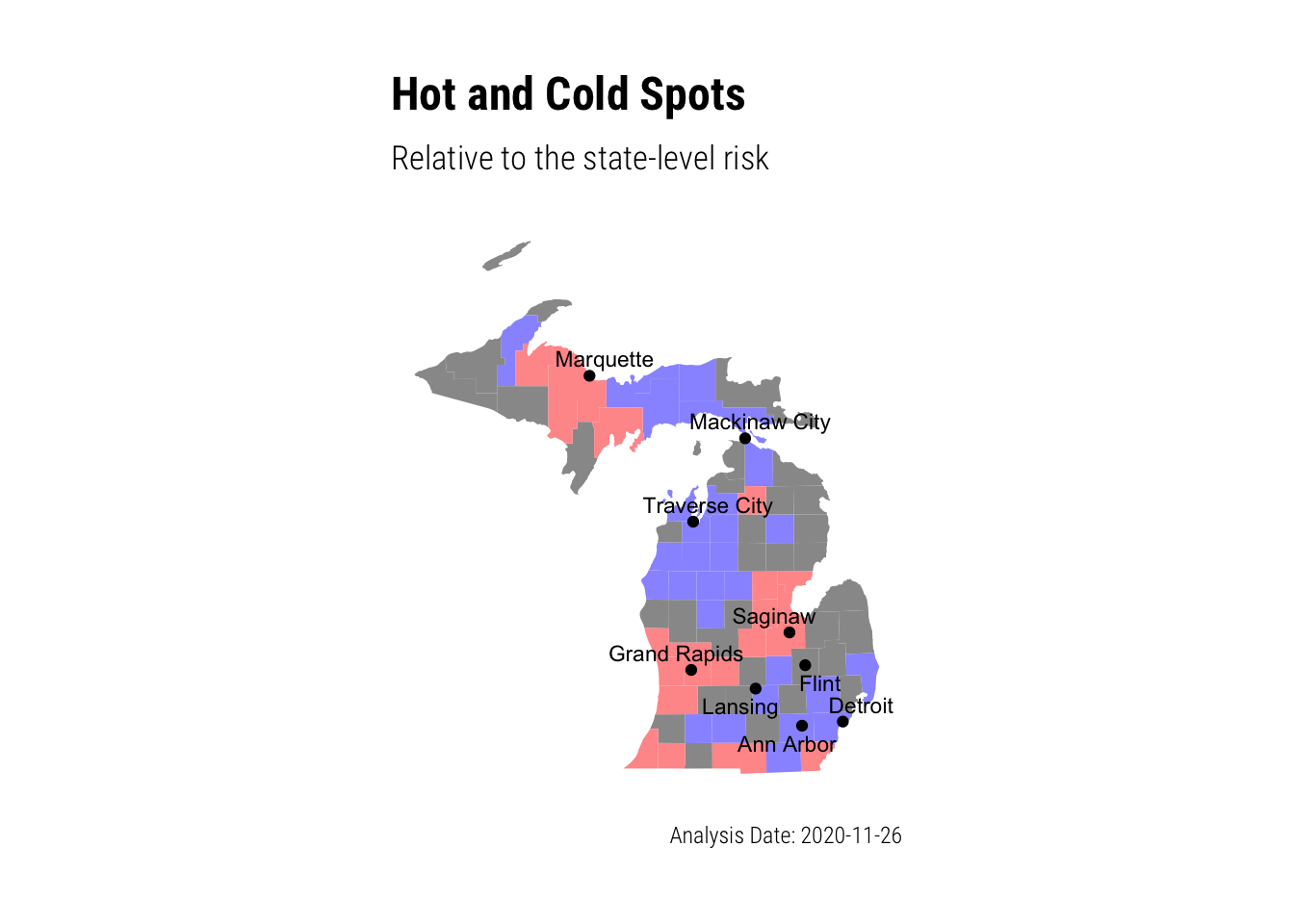
There are broadly three regions with elevated risk beyond the state-level: the Marquette region in the upper peninsula, the Saginaw region in central Michigan, and the Grand Rapids region in west Michigan. The counties in these areas have incidence rates that are significantly greater than the state-level. Additionally there are counties of elevated risk along the state’s southern border.

Summary

In this analysis I employed a Bayesian hierarchical modeling approach to calculate county-level incidence rates and identified COVID-19 hot spots – counties with significantly greater risk compared to the state-level. By using a Bayesian framework the model yields distributions of county-level incidence rates that could have produced the observed number of cases. Leveraging these distributions, we can better understand variation in county-level risk. These areas with elevated incidence rates may benefit from greater resources and interventions.