Rental Listings Part 2 - Exploratory Data Analysis
Mar 26, 2017 · 560 words · 3 minutes read
This is the second post in my Two Sigma Connect: Rental Listing Inquiries Kaggle competition series. The first post covered data import/processing and this post contains some of my exploratory data analysis.
Univariate Summaries
The dataset contains 49,352 RentHop listings. I began by taking a look at univariate summaries of continuous variables. I excluded ID variables such as listing_id and BoroCode. While regular quantiles are fine, I also looked at the 1st and 99th percentiles which can highlight Note: blogdown doesn’t seem to always play nice with htmlwidgets, so I used knitr::kable instead of DT::datatable.
| Variable | Min | 1st | 25th | Median | 75th | 99th | Max | St. Dev. | Missing |
|---|---|---|---|---|---|---|---|---|---|
| bathrooms | 0.0 | 1.0 | 1.0 | 1.0 | 1.0 | 3.0 | 10.0 | 0.5 | 0 |
| bedrooms | 0.0 | 0.0 | 1.0 | 1.0 | 2.0 | 4.0 | 8.0 | 1.1 | 0 |
| description_length | 0.0 | 0.0 | 339.0 | 563.0 | 808.0 | 1826.5 | 4465.0 | 394.0 | 0 |
| km_from_centroid | 0.2 | 0.4 | 1.8 | 3.2 | 5.4 | 15.1 | 8665.8 | 136.7 | 0 |
| latitude | 0.0 | 40.6 | 40.7 | 40.8 | 40.8 | 40.9 | 44.9 | 0.6 | 0 |
| longitude | -118.3 | -74.0 | -74.0 | -74.0 | -74.0 | -73.9 | 0.0 | 1.2 | 0 |
| price | 43.0 | 1475.0 | 2500.0 | 3150.0 | 4100.0 | 13000.0 | 4490000.0 | 22066.9 | 0 |
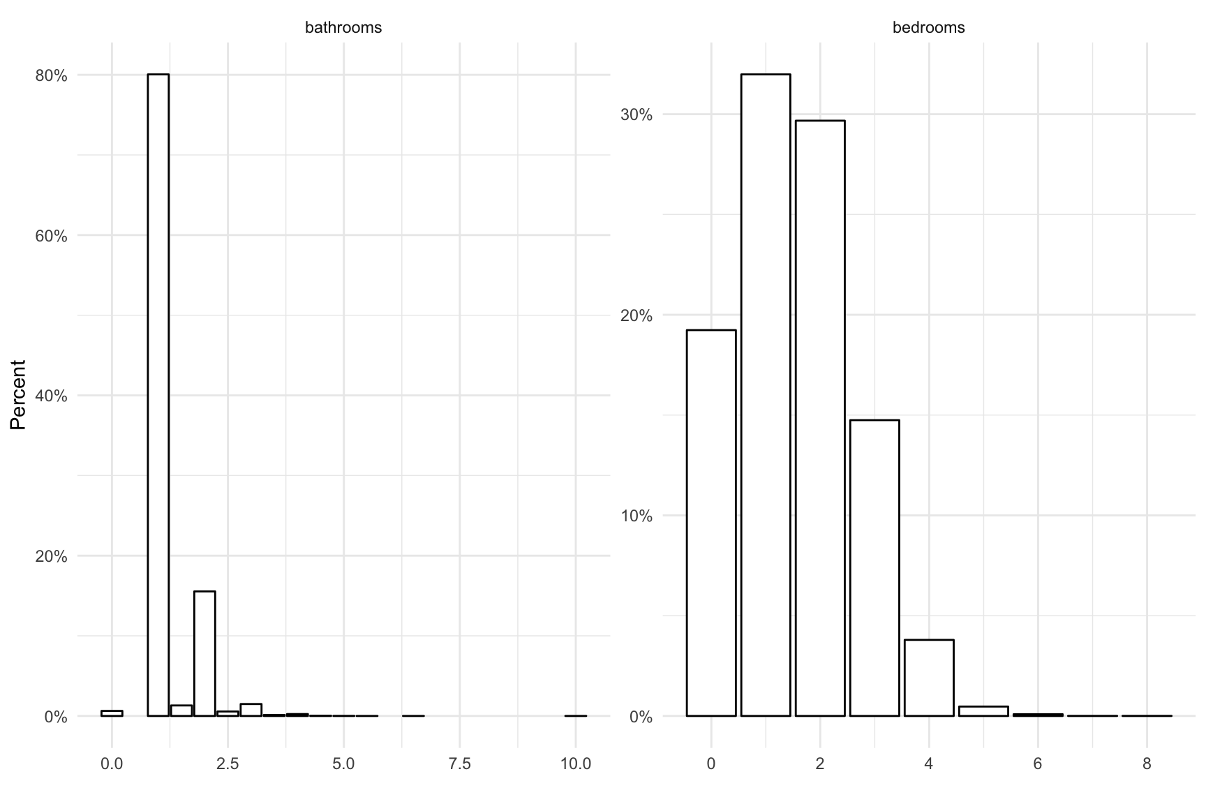
While bathrooms and bedrooms are numeric, I noticed they may behave more like ordinal categorical variables – most listings are for 1 or 2 bedroom apartments with a single bathroom. Since 99% of listings have 4 or fewer bedrooms and 3 or fewer bathrooms, it may be worth recoding these. Extreme values are evident for each variable (i.e. gaps between the 1st percentile and the minimum and/or the 99th percentile and maximum values).
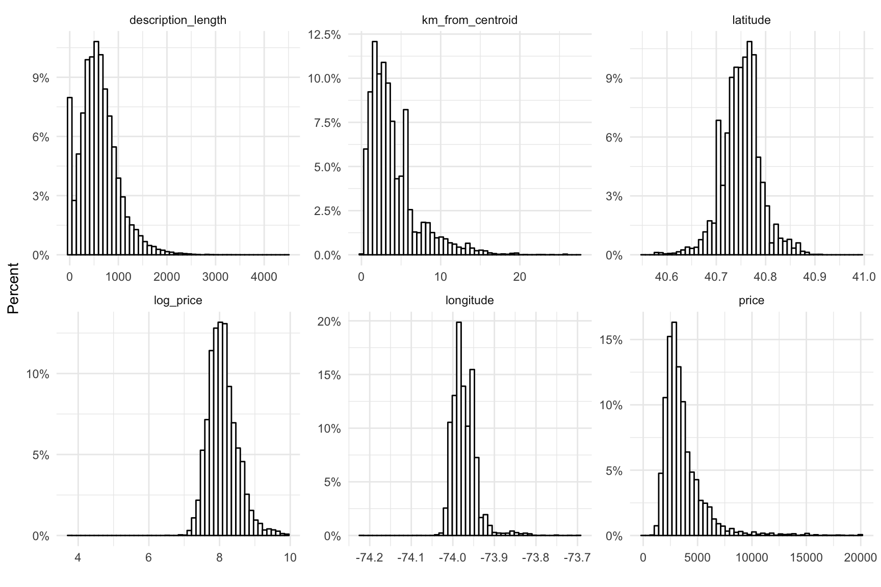
For the data visualization, I filtered out listings more than 30km from the data centroid (km_from_centroid <= 30) and with prices greater than $20,000 (price <= 20000) to improve visualization. Most listings have only a single bathroom and nearly 20% of the listings had no bedrooms (presumably studio apartments).
The listing description length appears zero inflated, with about 8% of listings having no description, and long tailed. Most listings are within several kilometers – a quick Google search shows that NYC is 789 \(km^2\), and \(\sqrt(789)=30\) so the distance distribution and my cutoff of 30 km seem pretty reasonable. Listing price is skewed right (surprise surprise) but nothing a log-transformation can’t fix.
Listing interest level was coded as a categorical variable (low, medium, and high), with most listings receiving low interest.
| interest_level | n | % |
|---|---|---|
| high | 3839 | 7.8 |
| low | 34284 | 69.5 |
| medium | 11229 | 22.8 |
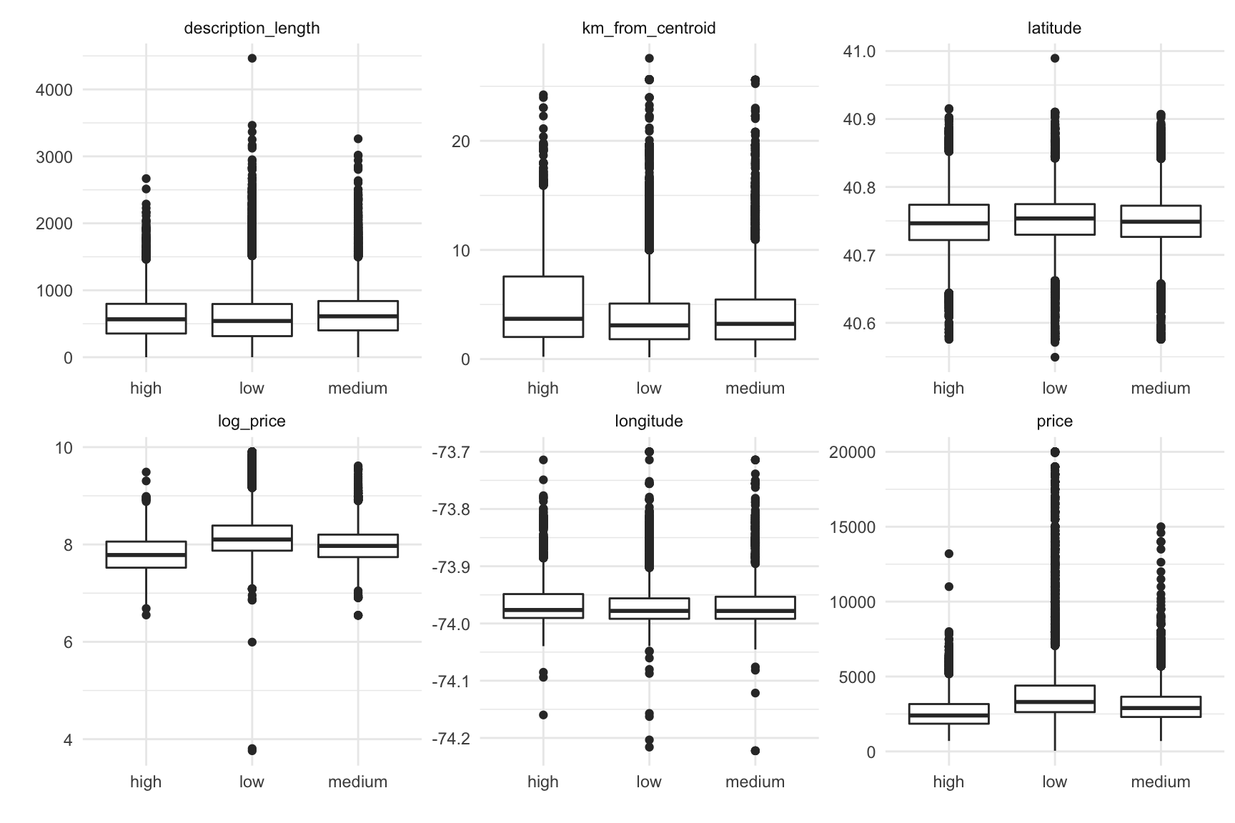
While I wasn’t really interested in the competition goal, predicting listing popularity, I decided to take a look at boxplots of each variable against listing interest level. There is quite a bit of variability, so there isn’t a single variable that really pops out as a driving factor. That isn’t too surprising since listing popularity is likely driven by a combination of factors.
Summary and Next Steps
This would be a good time to go back and construct additional features. I chose not to include the timestamp component, but I could easily see that datetime components (e.g. time of day, day of week) as influential factors. Additionally it could be useful to perform text mining on the actual descriptions, rather than just a simple character count, to see the impact of different keywords. I also didn’t do anything with the photos that were included – a simple photo count could help explain why some listings have a higher or lower rating.
Next up: mapping the data in Leaflet.